Neural Style Transfer Survey of Machine Learning Architectures

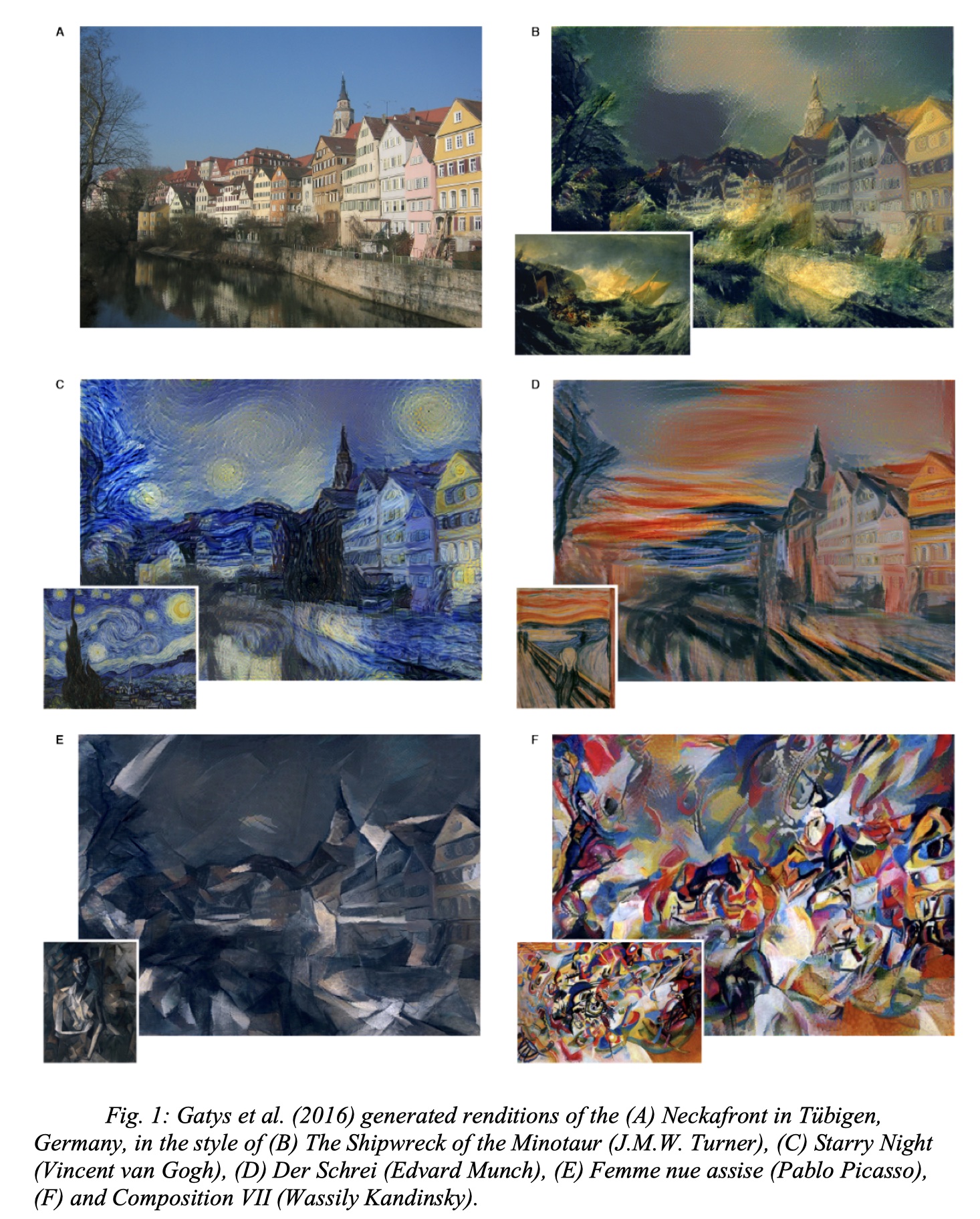
In computer vision, neural style transfer (NST) is a captivating technology that generates an image by imprinting the unique stylistic of one image onto the content of another image (Elgendy, 2020). Style transfer had been explored in the realm of image processing, but it consolidated itself as a recognized technique when Gatys et al. (2016) implemented a transfer algorithm using a deep convolutional neural network (CNN), achieving results far beyond anything prior. Using a VGG19 architecture, they transferred the authentic textures, color palettes, and unique characteristics of famous paintings onto a photograph (fig. 1). Subsequent research has led to improved results and various approaches that yield different outputs. Some experiments focused on improving resolution to the point of photorealism (Kim et al., 2021), while others focused on real-time execution (Johnson, 2016).

I set out to learn about this emergent medium, experimenting with different input images, pre-processing techniques, pre-trained CNN architectures, optimizers, and hyperparameters. I attempted to replicate previous NST efforts in deep learning (DL). It was my intention to achieve a real-time NST implementation that runs on a consumer-level laptop computer. This proved to be an ambitious task, and while I was able to make some progress towards this goal, I have not consolidated my progress into an output I am ready to deploy.

My NST experiments were successful. I attribute the differences to the approach I took when implementing my loss function, as well as the hyperparameters I experimented with, including optimizer type, the usage of exponential decay during optimization, activation layers used for extracting features, and the weight values assigned to each loss component.

Definitions

Chollet (2021) notes that the “activations from earlier layers in a network contain local information about the image, whereas activations from higher layers contain increasingly global abstract information” (p. 384).

With this in mind, we can define two recurrent keywords: content and style.

• Content: The content is the higher-level macrostructure of an image (e.g., dogs, buildings, people). Since the content tends to be global and abstract, it is to be expected that deeper layers of the CNN will capture these representations.

• Style: The style of an image encompasses textures, colors, and visual patterns at

various spatial scales (e.g., brush stroke directionality and width, color palettes, color gradients). 5 Because style exists at all scales of an image, its representations can be found in both shallow and deep layers of the CNN, meaning that layers in several depths must be considered to analyze the style of an image.

In NST, two images are provided as inputs: the one with the style of interest (style image), and the one with the content of interest (content image). The output image (combined image) applies the style of the style image to the content of the content image. Their relationship resembles modulation in digital signal processing (DSP), where a carrier signal (the content image) is modulated by a modulating signal (the style image).

Algorithm Outline

A general approach of the NST algorithm is as follows (Chollet, 2021, p. 385) :

1. A CNN simultaneously computes the layer activations for the style image, the content image, and the combined image. This CNN is a feature extraction model built from selected convolution layers that provides access to the layer activations across these layers.

2. The layer activations are used to define a loss function that needs to be minimized to achieve style transfer (Elgendy, 2020, p. 393):

 

total_loss = [style(style_image) – style(combined_image)] +

             [content(content_image) – content(combined_image)] +

             total_variation_loss

When comparing both the content representation of the content and combined images and the stylistic representation across multiple scales of the style and combined images, what is being compared are the feature activations at each chosen layer. However, it is worth noting that the styling activations are not directly compared. Prior to computing the mean square error, each style activation is processed through a spatial correlation matrix, the Gram matrix. The Gram matrix measures the similarity between a pair of feature representations at each layer: the style features of the style image vs. the style features of the combined image. Mathematically, the Gram matrix computes the inner dot product between a pair of vectors, which captures the similarity between the two. The more alike the two vectors are, the greater the dot product will be, resulting in a larger Gram matrix as well. This process captures the prevalence of different features across layers. Finally, the total variation loss component ensures that there is continuity between the regions across the image. Note that Gatys et al. (2016) did not implement a variation loss component in their original experiments.

3. Gradient-descent is used to minimize the loss function. This step adjusts the content of the combined image to better resemble the high-level features of the content image, while making the stylistic features of the combined image more like the ones of the style image.

Data

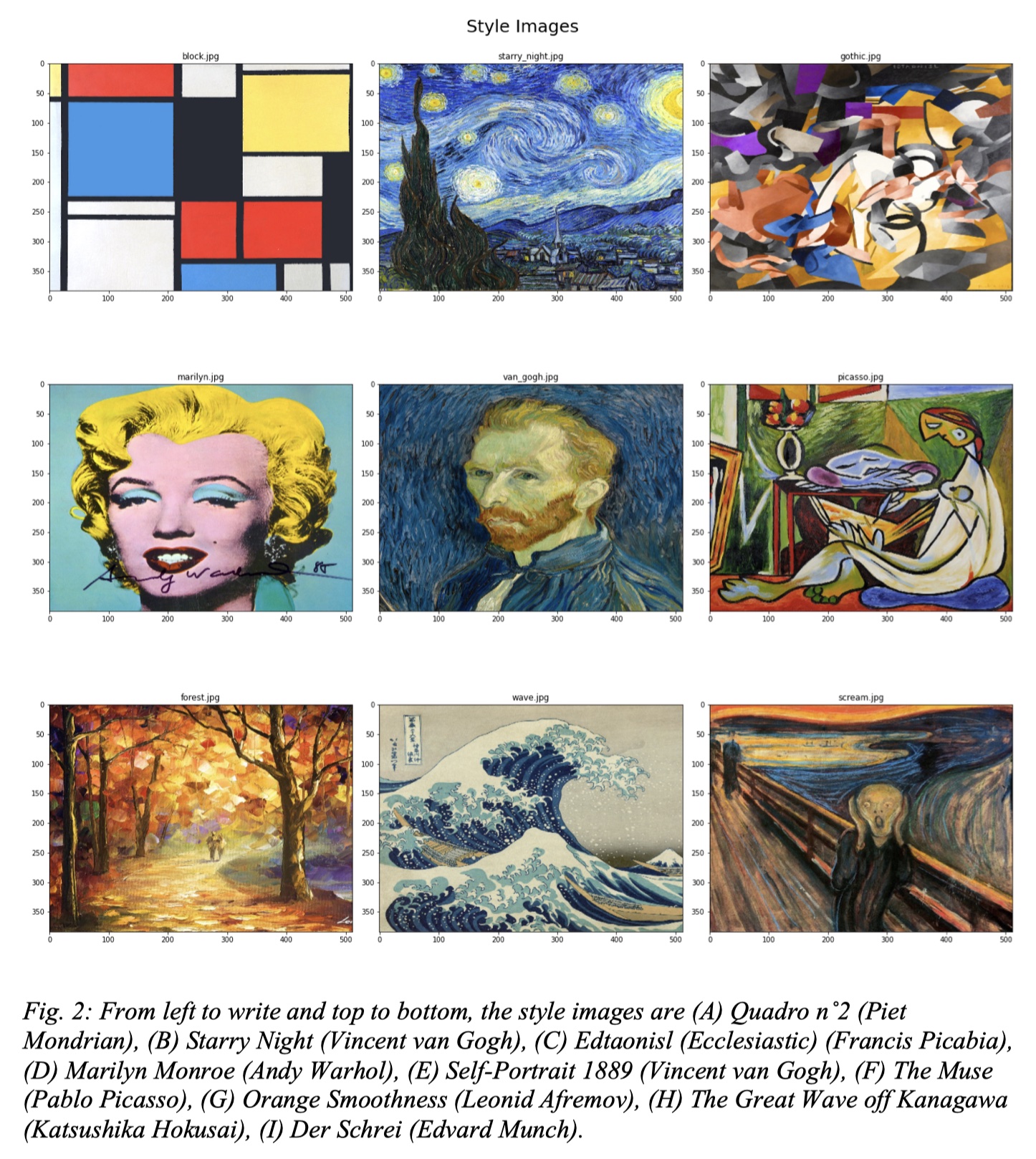
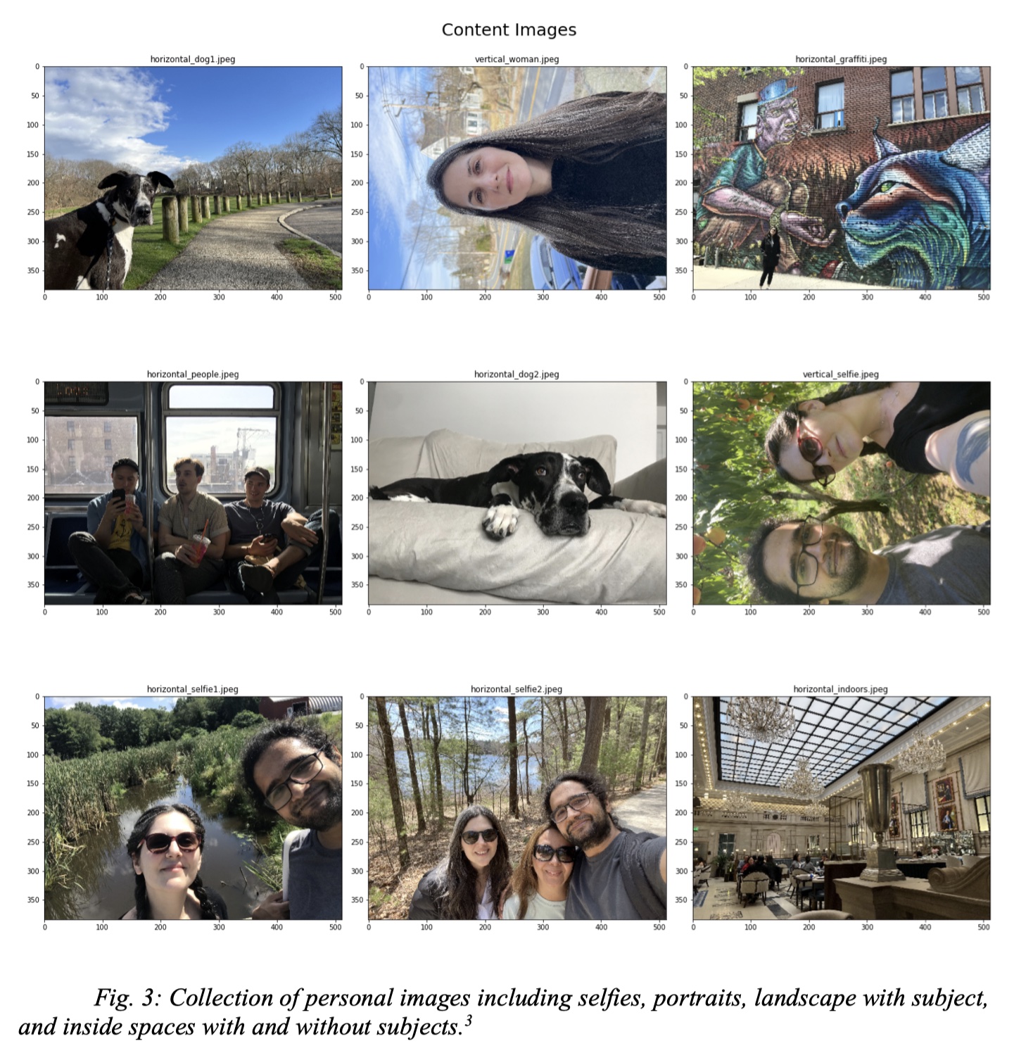
In general, NST does not require lots of data, but it needs a pre-trained CNN. This is because training the CNN from scratch would require enormous amounts of time, data, and resources. It is thus necessary to use a pre-trained model and discrete images. The images are separated into two categories: style images such as paintings (fig. 2), and content images such as photographs (fig. 3).

 

NST needs a trained model to extract image features, which are accessed by tapping into specific activation layers at different depths. I developed my implementation utilizing Keras’ VGG16 and VGG19 architectures, all using the pre-trained ImageNet weights

Pre-Processing

As differently sized images make the NST process more difficult, it is important to resize content and style images to make sure that their dimensionality is similar (Chollet, 2021). For this reason, I first made sure to resize both style and content images so that they all had the same dimensions.

According to the Keras implementation, different model architectures expect the input images to be in different formats. These formats are important achieving appropriate results from the model. Both VGG16 and VGG19 expect RGB images in range of 0 to 255 to be converted to BGR color space, and then zero-centered with respect to the ImageNet dataset (mean values of [103.939, 116.779, 123.68] for the BGR channels respectively). Understanding these preprocessing considerations are important for two reasons: incorrect image formats will yield incorrect results (which can be avoided by using Keras’ built-in preprocessing methods), and more importantly, knowing how to de-process the generated images so they can be in a standard RGB format will allow the algorithm to return usable media. Reverting the pre-processing is as simple as reversing each model’s steps one at a time.

Feature Extraction

It was fundamental to create a custom feature extraction model based on the different CNN architectures. This was done by choosing specific layers of these architectures and creating a new model via the various utility functions provided by Keras. This custom model extracts the features from the activation layers that will be used to calculate the previously defined loss function. As mentioned above, the loss function considers different stages of the CNN for the input images:

• A deep layer will be used in the portion of the loss function that compares the content image and the combined image. The smaller their difference, the more the combined image will embody the high-level features of the content image.
• Layers at different depths of the CNN will be used in the portion of the loss function that compares the style image and the combined image. This is because the stylistic features that of an image are present at all scales of the image, from low-level features (e.g., edges, corners), to mid and high-level features (e.g., stroke directionality, brush textures, color gradients).
• The optimizer applies the gradients that are computed using the loss function to the combined image, and thus makes a fundamental part of my feature extractor model.

Results and Findings

The results of my experiments were very successful, and I was able to transfer the stylistic features of a painting onto photogram with very aesthetically pleasing results! If you'd like to experiment with my code, it can be easily run on Google Colaboratory here.

Combined images from many well known paintings and "Dog in Landscape" utilizing a VGG19 architecture with a content activation layer in Block 5, Conv. 4.